Why are B-trees so widely used in databases?

I have spent quite some time researching how a database works internally and I thought to write about what I have learned so far. A database system consists of many components like the query planner, the query execution engine, the storage engine, the data replication and sharding mechanisms, etc. The key component is the storage engine, which determines how the data is represented, accessed and stored. It consists of several different components, but at the core of almost all database storage engines there is a data structure, named B-tree, around which all the other modules revolve. Let’s explore why is it so.

Data durability and its performance implications

A database management system processes and stores millions of records. With the purpose of maintaining a high processing speed, it can store the data in the main memory. But, we do not want to lose the data after a server restart due to a power outage, a server crash or a maintenance operation. So we have to ensure data durability. Therefore, we have to also store the data on a secondary storage, for example, on solid-state drives (SSD) or on hard disk drives (HDD).

Our first approach would be to store the records into a file. Then, when we want to find a record specified by its ID, we read the file sequentially until we find it. In the worst case, either when the searched record is located near the end of the file or when it simply does not exist, we will scan the entire file. This approach has one big problem though.

The secondary storage is several orders of magnitude slower than the main memory. For example, reading 64 bits non cached from the primary storage takes about 100 nanoseconds (ns), while reading a random block of 4 KiB from an SSD takes about 100 microseconds (µs) ¹. At a first glance, it seems that it is not that slow. But a CPU fetches data from main memory through a layered system of cache that reduces the average latency to a few nanoseconds. On the other hand, the latency of a secondary storage depends on multiple factors: access pattern (sequential or random), I/O size, I/O queue depth, I/O concurrency, storage capacity, etc. So the average latency of the secondary storage varies significantly depending on the type of the workload. Although the operating system as well as the secondary storage devices implement a caching system that improves the read and write performance, it does not bring it considerably closer to the read and write performance from the main memory. More than that, initially, the HDDs were the predominant secondary storage devices, which have a much worse performance than SSDs due to the limited speed of the spinning platters and the moving magnetic heads.

With our first approach and millions of records, it will take hours or even days to find the requested record.

Binary search tree

A second approach would be to keep the records sorted by ID in a file. Then, we can use the binary search algorithm to find the records. The time complexity of this algorithm is \(O(log_{2}{n})\), where n is the number of records. This means that if we have 1 million records, we need to access at most 20 records (\(log_2 10^6 \approx\) 19.93) to find the correct one. If the record size is less than or equal to 4 KiB, then the average latency of finding a record is 2 ms (\(20 \times 100 \mu s = 2000 \mu s = 2 ms\)). Not bad, but it quickly gets worse. Firstly, the size of a record is usually much higher than just 4 KiB, which increases the read latency. Secondly, we have to keep the records sorted in the file while they are inserted or deleted.

The simplest data structure that provides binary search and allows fast insertions and deletions is the binary search tree. Each node in the tree will contain the record ID, the record data and two references to the child nodes. Since we store the binary search tree on the secondary storage, the reference to a node will represent its location in the file and will consist of the file offset and the node size.

An example of a binary search tree is presented below. For simplicity, only the keys (record IDs) are illustrated to show the ordering relationship between them, even though a node contains both a key and its value. The same applies for all the other trees presented in this post, unless otherwise specified.

The minimum height of the binary search tree is \(log_2 (n + 1) - 1\), where n is the number of nodes in the tree. This follows from the structure of the tree. Each node can have at most two child nodes. So on the first level of tree we can have at most one node (the root), on the second level we can have at most two nodes, on the third level four nodes, on the forth level eight nodes and so on. It forms a geometric progression of the following form:

\begin{aligned} 2^0 + 2^1 + 2^2 + 2^3 + … + 2^h = 2^{h + 1} - 1 \end{aligned}

The total number of the nodes in the tree is the sum of all the nodes on each level:

\begin{aligned} n \le 2^{h + 1} - 1 \end{aligned}

Therefore, the minimum number of levels, that is, the minimum height of the tree is:

\begin{aligned} h \ge log_2 (n + 1) - 1 \end{aligned}

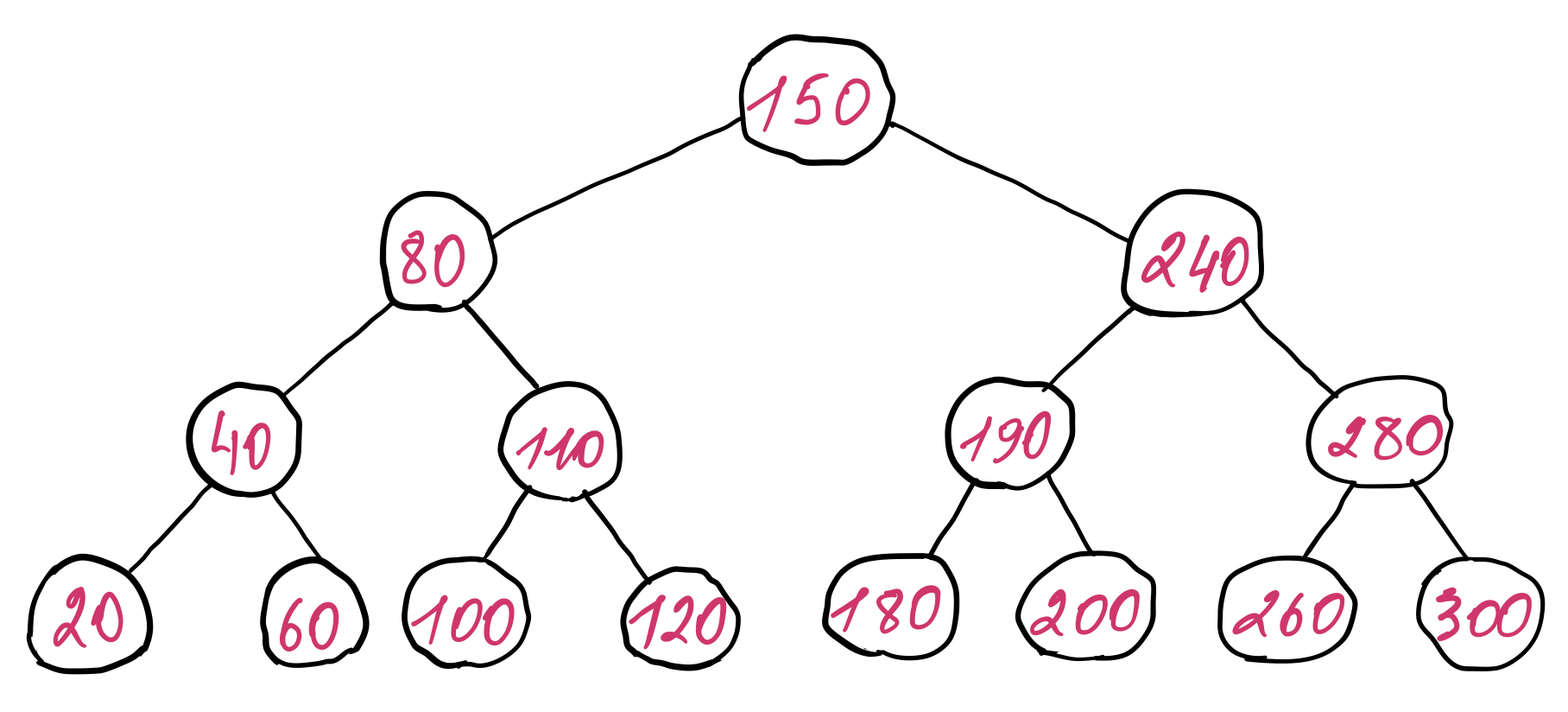
So the average time complexity of all three operations (search, insert and delete) is \(O(log_{2}{n})\). The insertion and deletion operations have to perform a binary search in order to determine where to insert or delete the record. But their worst time complexity is \(O(n)\). This is because the tree becomes unbalanced (i.e. the height of tree is greater than \(log_2 n \)) after arbitrary insertions and deletions. Furthermore, if we insert records that are already sorted, then the tree will degenerate into a linked list (each record will be inserted into one part of the tree leaving the other part empty). One example of unbalance of the above binary search tree depending on the order of insert and delete operations looks like the following:

As we can observe, when the binary search tree is unbalanced, many nodes have only a single child node. This leads to an increase of the height of the tree. Consequently, the time complexity of the binary search is no longer \(O(log_{2}{n})\), but somewhere between \(O(log_{2}{n})\) and \(O(n)\). In the worst case, when the tree is completely unbalanced, the binary search turns into a linear search. Hence this approach would degenerate to our first approach, which is scanning the entire file to find a given record.

There are multiple ways to keep the binary search tree balanced, that is, to keep the height of tree at its lowest value. Such trees are named self-balancing binary search trees. Some of the well-known self-balancing binary search trees are AVL tree and Red-black tree. They keep the tree balanced by tracking the degree of unbalance and performing several modifications on the structure of the tree after almost each insertion and deletion. When the tree is kept only in memory applying these transformations is cheap, but since we must also store the tree on the secondary storage, these transformations become very expensive. We will have to perform several additional reads and writes to change the references of adjacent nodes, such that the tree remains balanced. This will increase the overall latency of insertions and deletions.

Moreover, what if we want to store more than just one million records. With tens or hundreds of millions of records, the minimum height of the tree becomes a big multiplicative factor in the latency formula of an operation performed on the binary search tree.

One could think to keep an in memory representation of the binary search tree that holds only the locations of the nodes in the file, essentially building an index. Then the balancing operations are much cheaper. But the index size is directly proportional to the data size, meaning that a larger amount of data produces a larger index size. Eventually, we will want to store the index on the secondary storage to avoid expensive creation process each time the database server starts. Also due to memory constraints, we may not be able to keep the entire index in memory. At the end of the day, we end up with the same kind of problem. However, as we will see a bit later, solving the original problem will enable a significant improvement of the index performance as well.

In a nutshell, all the problems of storing the records on the secondary storage structured as a binary search tree revolve around its height. In particular, as we have discussed, we have the following problems:

• the binary search tree requires balancing operations after almost each insertion and deletion to keep its height at the minimum value; these operations are quite expensive when performed on the secondary storage
• the minimum height of the binary search tree becomes quite large with hundreds of millions of records when placed in the context of how many nodes have to be accessed to fulfil a tree operation.

B-tree

Let’s play with the structure of the binary search tree keeping in mind the problems of the height and see if we can do something about them. The level of a node is the number of edges from it to the root. The root node has level zero. The height of a node is the length of the longest path of edges to a leaf from that node. A leaf node has hight zero. The height of the root node is the height of the tree. It is similar to the level of a node, it is just counted in the opposite direction.

A tree is composed of smaller subtrees. Let’s identify subtrees of an arbitrary height in our binary search tree example. If we choose the height to be one, we can find the following subtrees:

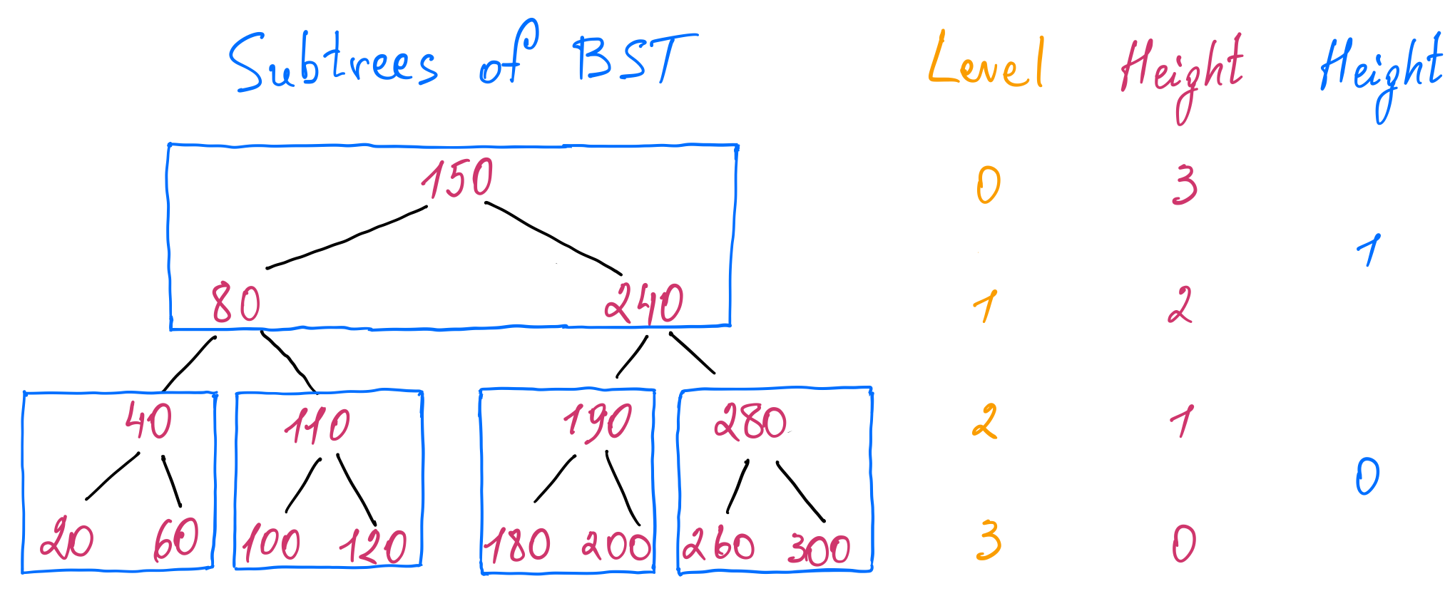
We can make an interesting observation that if we consider each subtree as being a node, we obtain a new tree where the total number of levels is reduced by half and the height of the tree is also reduced by half. We can think of it as creating a tree of a tree, where each node of the new tree references a subtree of the old one.

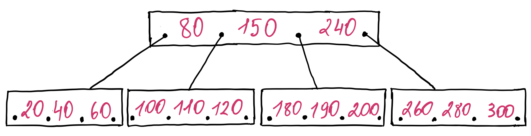
Also, a node has more than two children. All keys of the most left child node are smaller than the first key of the parent node. The keys of the second child node have values greater than the first key and smaller than the second key of the parent node and so on. Lastly, the keys of the most right child node have values greater than the last key of the parent node. If we store the entries of a node in a sorted list for simplicity, we get the following tree:

The tree we ended up with is a form of a B-tree. In fact, it is a generalization of the binary search tree. It was invented by Rudolf Bayer and Edward M. McCreight while researching how to organize and maintain a large index for a dynamic random access file at Boeing Research Labs.

Great, but there are still a lot of questions:

• why is the number of levels and the height reduced by half?
• what is the relationship between the height of the old subtree and the height of the new tree?
• if we choose the height of the subtree to be 10, by how much is the height of the new tree reduced?
• how the search algorithm is affected?
• how do we keep the tree balanced?

Let’s try to answer these questions one by one!

Searching for a key

We can formalize the relationship² between the keys of the nodes to get a better picture of how the search algorithm would work. Let \(k\) be the searched key, \(p_i\) be the pointer to a node i, \(P(p_i)\) be the node with \(l\) pointers holding the \(p_i\) pointer. Let \(K(p_i)\) be the set of keys of the nodes of that maximal subtree for which the \(P(p_i)\) is the root. Then we define the following relationships:

\begin{aligned} &\forall k\in K(p_0), k \lt k_1 \newline &\forall k\in K(p_i), k_i \lt k \lt k_{i + 1}, i = 1, 2, …, l - 1 \newline &\forall k\in K(p_l), k_l \lt k \end{aligned}

Given these relationships, it is easy to see how the search algorithm works. When we search for a key \(k\), we start with the first node in the tree and find the key that is equal or smaller than \(k\). If the found key is equal to the searched one, we stop and return the record associated with that key. If the key is smaller than \(k\), we go to the child node referenced by the pointer associated with that key and the process repeats. It resembles the binary search algorithm. The difference is, when using the binary search to select a node to go to, there are two choices, we can go either to the left or to the right depending on the result of the key comparison. When searching through a B-tree, we select a child node to go to from the range of keys present on the current node. This selection can be performed either via a linear search or a binary search.

Balancing operations

How many entries a node should have? How does it influence the height of the B-tree? If each node contains only one entry, then the B-tree becomes a binary search tree. The more entries a node has, the smaller the height of the tree. Therefore, to ensure that the B-tree does not degenerate into a binary search tree, we can establish a minimum number of the entries per node. What value should it have? To answer this question, we have to find out how the insertion and deletion operations work.

We want the B-tree to remain balanced after arbitrary insertions and deletions, to preserve its height at the minimum value. So we can establish another property of the B-tree, which is, each path from the root node to any leaf node has exactly the same length. Keeping this property in mind, let’s explore how the insertions and deletions would work in a B-tree.

Inserting a new entry in a B-tree

To insert a new entry, we must first find the node where the new entry should be added by searching through the tree. If the searched entry is not present in the tree, then the node where we have to insert the new entry will always be a leaf node. Once we found that node, we can perform one of the following steps:

• if the node contains fewer than the maximum allowed entries, then we insert the new entry in this node, keeping the node entries sorted

• if the node is full, then we split it evenly into two nodes in the following way:

  • find the median entry from the set of all entries of the node including the new one
  • put the entries less than the median into the first node
  • put the entries greater than the median into the second node
  • insert the median entry into the parent node which would reference the two new nodes. This can cause parent node to split too, and so on. If we arrive at the root node and it is also full, then we create a new root node above it, increasing the height of the tree. Therefore, a B-tree always grows from the root.

We could have added a new leaf node under the found one and insert the new entry there. But that would create an imbalance in the tree, breaking the invariants of equal length of all paths from the root node to any leaf node, and the minimum entries per node (we certainly do not want to have only one entry in a non-root node).

When the node split reaches the root node, we create a new root node with a single entry in it. Therefore the minimum entries in a root node is one. What about the other nodes? Well, we have to make sure that when we split a node, each of the resulting nodes must have at least the minimum entries. One good way of achieving this is to ensure each non-root node is half full. That is, if we let \(k\) be the minimum number of entries per node, then the maximum number of entries per node must be \(2k\). Together with the new entry that will be inserted, we have \(2k + 1\) entries. From these, the first \(k\) entries are put into the first node, the entries from \(k + 2\) to \(2k + 1\) are put into the second node, and the median entry, that is, the (\(k + 1\))th entry is inserted into the parent node.

Deleting an entry from a B-tree

To delete an entry from the B-tree, we must locate it first. Once found, we perform the following steps:

• if the entry is on a leaf node, then we just delete it

• otherwise we have to find a replacement entry which will reference the left and right subtrees of the current entry. There are two options: we can either select the smallest entry from the right subtree or the largest entry from the left subtree, because only these two entries can satisfy the ordering constraints of the keys in the tree. Both of them can be found on the leaf nodes of the respective subtrees. It is important to note that once we choose an option, we should stick with it for a given B-tree. So for example, we remove the smallest entry from the right subtree and put it in the place of the entry to be deleted.

Deleting an entry can cause the respective node to have fewer than the minimum number of entries (\(k\)), a situation known as underflow. To keep at least the minimum established number of entries per node, we must rebalance the B-tree in the following way:

• if the sum of the entries of the node from which the entry was removed and one of its adjacent nodes from the same parent is less than or equal to \(2k\), then we simply merge the two nodes and remove one entry from the parent node. As a consequence, the parent node can have fewer than \(k\) entries and the entire process repeats. It can propagate up to the root of the tree, decreasing its height. Therefore, a B-tree also shrinks from the root.

• if this sum is greater than \(2k\), then we can equally redistribute the entries of both nodes among them. Since the entries of the two adjacent nodes are already sorted, we just move a sufficient amount of entries from the node with more than the minimum number of nodes (\(k\)) to the other node and update the parent node’s entry that points to these two child nodes. Redistributing entries among two nodes does not propagate. The parent node is modified, but the number of entries remains the same.

In comparison with the binary search tree where the balancing operations occur almost on every insertion and deletion, the balancing operations in a B-tree do not occur so often with a larger capacity of entries per node.

Height of the B-tree

Now that we have a better understanding of how the B-tree works, let’s determine its height. We want to express the height of the B-tree in terms of the number of entries. Since each node has more than one entry, we have to first calculate the number of nodes in a B-tree, then the number of entries and finally determine the height of the B-tree.

A node has a minimum of \(k + 1\) and a maximum of \(2k + 1\) children. The root node has at least \(2\) and at most \(2k + 1\) children. Therefore, we have a minimum and a maximum number of nodes in a B-tree. Let’s first calculate the minimum number of nodes. At the level zero, we have one node, the root. It has a minimum of two children, so at the level one, we have two nodes, each having \(k + 1\) children. At the level three, we have \(k + 1 \) nodes from the first parent and \(k + 1 \) nodes from the second parent and so on:

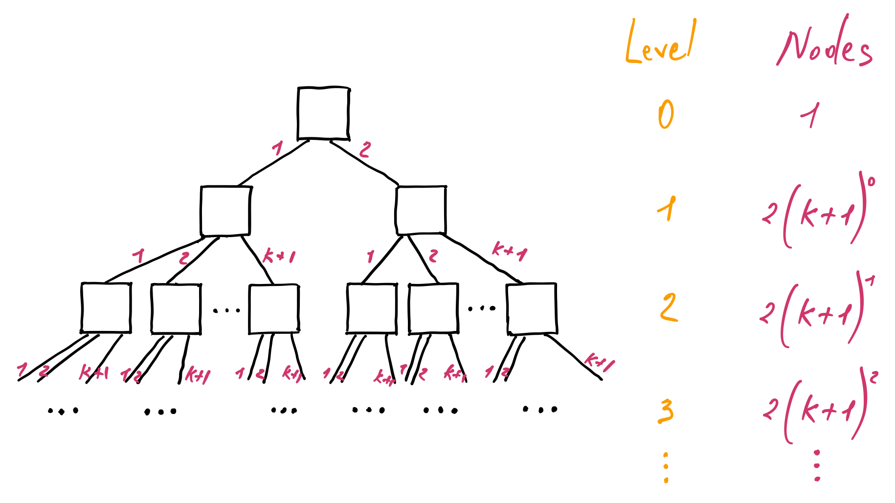
We can notice that both subtrees from the level one downwards are equivalent. Hence we can calculate the number of nodes for one of the subtrees and then multiply it by two to get the total number of nodes. Also, as we go from one level to the other, the sum of the number of nodes forms a geometric progression similar to the one we have seen when we have calculated the height of the binary search tree. Applying the same formula, we get the minimum number of nodes in a B-tree:

\begin{aligned} N_{min} & = 1 + 2 ((k + 1)^0 + (k + 1)^1 + (k + 1)^2 + … + (k + 1)^{h - 2}) \newline & = 1 + 2 \sum_{i=0}^{h - 2} (k + 1)^i \newline & = 1 + \frac{2}{k} ((k + 1)^{h - 1} - 1) \end{aligned}

Using a similar approach, we can calculate the maximum number of nodes in a B-tree. At the level zero, we have the root node that can have at most \(2k + 1\) children. As a result, at the level one, we have at most \(2k + 1\) nodes. At the next level, we have \(2k + 1\) nodes from each of the \(2k + 1\) parents, and so on:

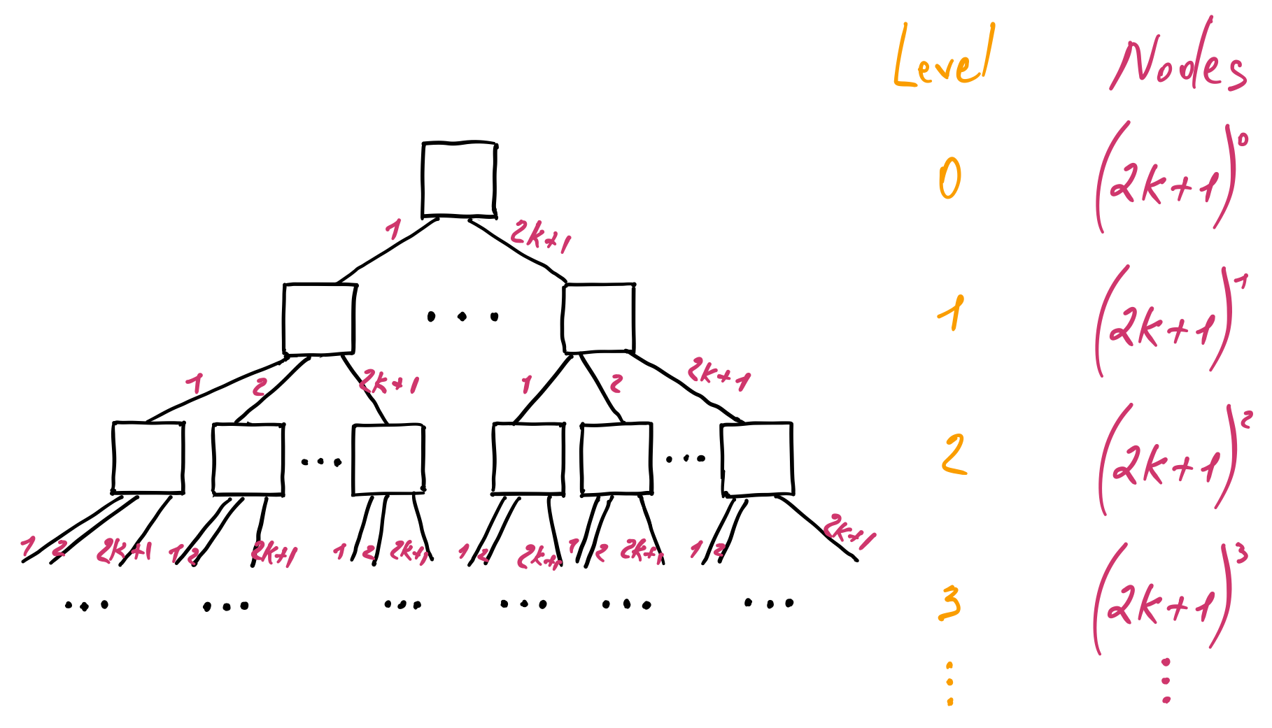
It forms another geometric progression. Applying its formula, we get the maximum number of nodes in a B-tree:

\begin{aligned} N_{max} & = (2k + 1)^0 + (2k + 1)^1 + (2k + 1)^2 + … + (2k + 1)^{h - 1} \newline &= \sum_{i=0}^{h - 1} (2k + 1)^i \newline & = \frac{1}{2k} ((2k + 1)^h - 1) \end{aligned}

We already know the minimum and maximum number of nodes in a B-tree, so determining the minimum and maximum number of keys in a B-tree is easy. We just have to multiply the number of keys per node with the total number nodes. Special care must be taken when calculating the minimum number of keys though, because the root node can have at least one key. Therefore, the minimum number of keys in a B-tree is one key in the root node plus the number of keys per node starting from the level one multiplied by the total number of nodes from the level one downwards:

\begin{aligned} I_{min} & = 1 + k (N_{min} - 1) \newline & = 1 + k (\frac{2}{k} ((k + 1)^{h - 1} - 1)) \newline & = 2(k + 1)^{h - 1} - 1 \end{aligned}

The maximum number of keys in a B-tree, given the number of nodes, is:

\begin{aligned} I_{max} & = 2k N_{max} \newline & = 2k (\frac{1}{2k} ((2k + 1)^h - 1)) \newline & = (2k + 1)^h - 1 \end{aligned}

Then, it follows, that the height of the B-tree is:

\begin{aligned} \log_{2k + 1}(I + 1) \le h \le \log_{k + 1}(\frac{I + 1}{2}) \end{aligned}

This is the relationship we were looking for to understand why the size of the B-tree we have obtained after applying certain transformations to the binary search tree, was reduced by half. We had 15 entries in the binary search tree. Its height was 3 (\(log_2{(15 + 1)} - 1 = 3\)). Next we have created a B-tree, where each node had 3 entries representing a subtree of the binary search tree. Using the above formula, we calculate the height of the B-tree to be 1 (\(\lfloor log_4{15} \rfloor = 1\)). Hence, the height was reduced by half, from 3 to 1.

Given this relationship, we can deduce the time complexity for all B-tree operations (search, insert and delete) as it is shown in the following table:

Algorithm	Average	Worst
Search	\(O(log_{b}{n})\)	\(O(log_{b}{n})\)
Insert	\(O(log_{b}{n})\)	\(O(b\log_{b}{n})\)
Delete	\(O(log_{b}{n})\)	\(O(b\log_{b}{n})\)

The average time complexity of all its operations is \(O(log_{b}{n})\), where \(n\) is the number of entries in the tree and \(b\) is the minimum branching factor, that is, it is the minimum number of child nodes a node can have, which is \(k + 1\). The worst time complexity of insertions and deletions is \(O(b\log_{b}{n})\) because in the worst case we have to perform balancing operations, shuffling \(O(b)\) entries at each level, from a given node (leaf or non-leaf) up to the root, which is \(O(log_{b}{n})\).

If we have one million records and store 64 entries per node, then we need to read only 4 nodes from the file to find the right record (\(log_{65}{10^6} \approx 3.3\)). This is a huge improvement compared to a binary search tree where we had to read 20 nodes to find the right record. Hold on! Storing 64 entries per node makes the node size much larger. Yes, indeed. But performing a few read operations with a large block size each, yields a better disk utilization and lower latency than performing a large number of random reads with a small block size. On the other hand, we cannot read very large blocks of data at once, since we may not have enough memory capacity to hold even one of it. Also, the proportion of data we would read with respect to the amount of data we need would be very high.

Therefore, we have to establish a maximum size for a node. That imposes a limit on the maximum number of entries a node can have. Since a B-tree keeps not only the key and two pointers to the corresponding child nodes, but also the associated value with that key in the node, the size of the value should be quite small to allow a large number of entries per node and not exceed the maximum node size. One way to keep the size of the value quite small is to store an address of the record located in another file. We would have to manage two files, one which stores the B-tree representation and the other would store the actual records. But there is a better way!

B+ tree

Nowadays, most databases use an improved version of the B-tree, named B+ tree. It minimizes the size of the non-leaf (internal) nodes by keeping only the keys and the pointers to the child nodes. Only the leaf nodes contain the keys and their associated values (records). This implies that some of the keys will be duplicated in the tree. Additionally, each leaf node contains a pointer to the next leaf node forming a linked list of leaf nodes. This is very useful for range queries or full table scans, because once the starting key is found we can just navigate directly through the leaf nodes without needing to traverse the internal nodes multiple times.

Taking the example of the above B-tree and transforming it into a B+ tree looks like this:

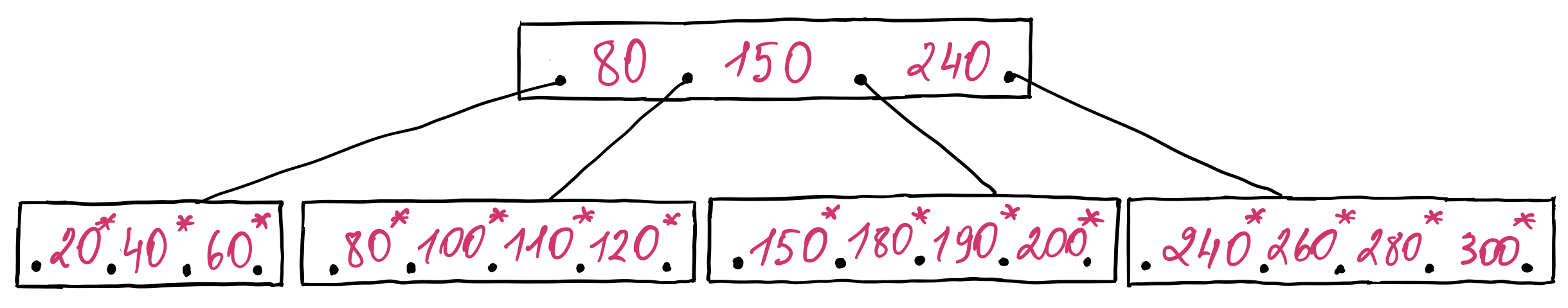
The keys from the leaf nodes are marked with an asterisk to indicate that an entry consists of the key and the associated information with that key. As a consequence, the minimum or maximum key of the leaf node is also present in its parent internal node. This slightly changes the relationships between the keys of the B+ tree, compared with those of the B-tree. Using the same notation, we can define these relationships in the following way:

\begin{aligned} &\forall k\in K(p_0), k \lt k_1 \newline &\forall k\in K(p_i), k_i \lt k \le k_{i + 1}, i = 1, 2, …, l - 1 \newline &\forall k\in K(p_l), k_l \le k \end{aligned}

Note that we can define the equality relationship either on the left or on the right side of a subtree, that is, we can either keep the minimum key of the right leaf node in its parent, or we can keep the maximum key of the left leaf node in its parent. It is important that once a convention is established, it must be maintained for a given B+ tree.

Searching for a key in a B+ tree works similarly as the search in a B-tree, the difference being that we traverse the B+ tree until a leaf node is reached following the relationships of the keys. If the searched key is found in the leaf node, then we return its value, otherwise the key is not present in the tree.

Inserting an entry in a B+ tree

Inserting an entry in a B+ tree is quite similar to inserting an entry in a B-tree. We first find the leaf node where the new entry should be inserted and then add it there. If an overflow occurs, then we have to split the leaf node. Since a leaf node keeps both the keys and their associated values, the median key cannot be moved into the parent node, it is copied instead. Splitting an internal node follows the same rules as splitting a node in a B-tree.

Deleting an entry from a B+ tree

Deleting an entry from a B+ tree is also similar to deleting an entry from a B-tree. As usual, we first search for the key record to be deleted, which will end in a leaf node. Then we delete the entry if it exists. Deleting an entry from a node can cause an underflow, which we can fix as follows:

• if the sum of the entries of the node from which the entry was removed and one of its adjacent nodes is less than or equal to \(2k\), then we simply merge the two leaf nodes and remove one key entry from the parent node. This can propagate up until to the root node, at which point the B+ tree shrinks in height.

• if this sum is greater than \(2k\), then we can equally redistribute the entries among the two leaf nodes and update the corresponding key entries from the parent node.

What shall we do if the key is also present in one of internal nodes (propagated during a node split)? We could try to delete it. In practice though, it is left there, because it does not affect the search operation. Eventually, after a number of merging nodes or key redistribution operations, those keys will be removed.

Data compression

We can reduce the size of the keys and values stored on secondary storage even further by using data compression techniques! Some of the most popular techniques are:

• key prefix compression reduces the node size by storing the common key prefix only once per node. For example, let’s say we have the following keys: extraordinary, extraterrestrial and extraction. Their common prefix is “extra”. If we store this prefix only once per node we save a few bytes, which allows us to fit a few more keys on the same node. The downside is that during a key lookup if the node is read from the secondary storage we have to decompress a number of keys to perform the search. That requires additional CPU cycles and memory. Therefore, this type of compression should only be applied when the number of bytes saved per key is much higher than cost of decompressing the key. In practice, this technique is mostly used only for the leaf nodes. B-trees that implement the key prefix compression are named prefix B-trees³.

• key suffix truncation reduces the node size by removing the trailing bytes unnecessary to perform the search. This technique is only used for internal nodes. When a leaf node is split, we copy the median key into the parent internal node which acts as a separator between the two leaf nodes. Instead of copying the median key, we can put the shortest string that separates the highest key of the left node from the lowest key of the right node. The suffix truncation is applied only when a leaf node is split, because a key in the internal node must guide the search not only to the correct internal child node, but also to the correct leaf node. Applying this technique when an internal node is split, may result in the search being guided to the wrong subtree.

• dictionary compression reduces the leaf node size by storing identical values only once per node.

• page compression reduces the node size by compressing the node’s data before it is stored on the secondary storage. It is important to use lossless data compression algorithms that provide high compression speeds and reasonable compression ratio to minimize the CPU consumption. Among the most widely used algorithms for this purpose are snappy and lz4.

• variable-length integer encoding reduces the node size by encoding node’s metadata, which consists of integer values, in a way that uses only as many necessary bytes as possible. For example, the pointers to the child nodes may be represented as two integer values, one representing the offset in the file and the other the node size. If these values are stored as 32-bit unsigned integers, then the values up to 255 need only one byte of space (the least significant byte), the other three most significant bytes are just zeros. We can eliminate the zero bytes by applying a variable-length integer encoding, thus reducing the node size.

Due to the variable length of the keys and values as well as the usage of the data compression techniques, it is hard to estimate a minimum and maximum value of entries per node. So in practice, we establish a minimum and maximum node size ensuring that its size is sufficient enough to store many entries per node minimizing the height of the B+ tree. Since the leaf nodes store both keys and values, they have a different minimum and maximum node size than internal nodes. Usually, the maximum size of the internal nodes is set as a multiple of the OS memory page, like 4 KiB, 8 KiB, etc. The maximum size of the leaf nodes is much larger: 64 MiB, 256 MiB or even 512 MiB. For this reason, the words node and page are interchangeable in the context of B-trees. Then the minimum node size is specified as a proportion of the maximum node size. For example, to ensure a node size is half full, we set the minimum node size to be 50% of the maximum node size.

Height of the B+ tree

The height of the B+ tree is defined by the same relationship as the height of the B-tree. Generally, since we store more keys in the internal nodes (in the order of hundreds), the height of the B+ tree is smaller than that of a B-tree.

Having 132 entries per node allows us to keep 300 million entries in a B+ tree with a height of just 4 (\(log_{133}{(3 \times 10^8)} \approx 3.99 \)). We will have to access the secondary storage four times to find the searched record. More than that, when the nodes of the first two levels are cached in main memory, the number of accesses is reduced to two. If reading an internal page of 4 KiB takes about a 100 microseconds and reading a leaf page of 128 MiB takes approximately 2-3 milliseconds, then we can find a given record in just a few milliseconds.

The time complexity of the B+ tree operations is shown in the table below:

Algorithm	Average	Worst
Search	\(O(log_{b}{n})\)	\(O(log_{b}{n} + log_{2}{L})\)
Insert	\(O(log_{b}{n})\)	\(O(M\log_{b}{n} + log_{2}{L})\)
Delete	\(O(log_{b}{n})\)	\(O(M\log_{b}{n} + log_{2}{L})\)

The search operation has \(O(log_{b}{n} + log_{2}{L})\) time complexity in the worst case, because we have to search through \(O(log_{b}{n})\) internal keys and perform a binary search tree on the leaf node with \(L\) entries. Insertion and deletion operations have the time complexity of \(O(M\log_{b}{n} + log_{2}{L})\) in the worst case, because inserting or deleting an entry requires a search operation first. Additionally, we have to perform balancing operations, shuffling \(O(M)\) entries at each level, from a given node (leaf or non-leaf) up to the root, which is \(O(log_{b}{n})\) in the worst case.

Summary

In this post we have explored why are the B-trees so widely used by database storage engines to organize the records. We have started by defining our goal which was to ensure that the data we store is durable. Then we have found out that the secondary storage devices are orders of magnitude slower than the main memory, which led as to the data organization problem. We have briefly gone through a naive solution that did not scale with respect to the amount of stored data. Next, we have analyzed whether the binary search tree structure would help us. Although it turned out to be a considerably better solution than the previous one, the height of the binary search tree is quite high with huge amounts of records, preserving the operation latency at a very high value. Additionally, the balancing operations required at almost every insert and delete operations made things even worse.

Then, thinking about how we can solve the problems of the binary search tree, we have arrived at a new data structure, B-tree. It allows keeping hundreds of millions of records at a very small height and with less frequent balancing operations, which significantly reduces the operation latency. However the values can be quite large which limits the number of entries stored per node. In order to further reduce the B-tree height, we have analyzed an improved version of B-tree, named B+ tree, which is used by the majority of the modern database systems. The B+ tree keeps only the keys in the internal nodes and both keys and values in the leaf nodes, enabling the internal nodes to store much more entries than a B-tree, which in turn reduces its height.

Time complexity of the B+ tree and B-tree is quite close to that of the binary search tree, asymptotically they are the same. But the B-trees take advantage of the properties of the secondary storage devices, which are: reading and writing randomly a chunk of 4 KiB of records, or reading and writing sequentially a large chunk of 64 MiB of records is much faster than reading and writing individual records one at a time. The number of accesses to the secondary storage is much smaller and thus the cost of a B-tree operation is substantially smaller than that of a binary search tree.

What does B in B-tree stands for? Rudolf Bayer and Edward McCreight have never explained it, but Edward McCreight has said:

“the more you think about what the B in B-trees means, the better you understand B-trees.”

Let’s see what we have learned about B-trees:

• a B-tree is a generalization of the binary search tree
• a B-tree is a self-balancing tree
• a B-tree has a branching factor much greater than that of a binary search tree, which plays a key role in minimizing the height of the tree
• the branching factor of the B-tree represents the base of exponentiation and logarithm used to determine the number of entries and the height of the B-tree
• B-tree was invented by people working at Boeing Research Labs
• the name of the one of the inventors is Rudolf Bayer
• tress that have a B-tree at their base and include improvements, like B+ tree and B* tree, are commonly called the family of B-trees.

However, we have just explored the most essential aspects of B-trees. We have not explored how B-tress handle duplicate key entries, compound keys and bulk insert. More importantly, we have not investigated how records are updated in a B-tree. This would be the subject of another post.

---